
The Data output from web scraping isnt always clean and ready to be used/analysed. In this tutorial we will show you out tips and tricks t
By Victor Bolu @February, 7 2023

Web scraping is an automated method used to extract large amounts of data from websites. The data scraping usually is unstructured. So, cleaning of this scraped data is necessary to convert the unstructured data into structured form. From another perspective, spending time cleaning up messy data can fill the large gaps that your processor will experience when waiting for it to be downloaded from its host.
This section covers several useful clean-up operations of scraped data in an Excel or Google sheet
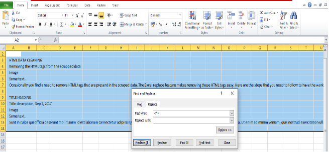
Occasionally you find a need to remove HTML tags that are present in the scraped data. The Excel replace feature makes removing these HTML tags easy. Here are the steps that you need to follow to have the work done:
Step 1: Select the cells that contain the HTML and then click CTRL+H or select Editing(Find and select)> Replace as indicated by arrow mark.
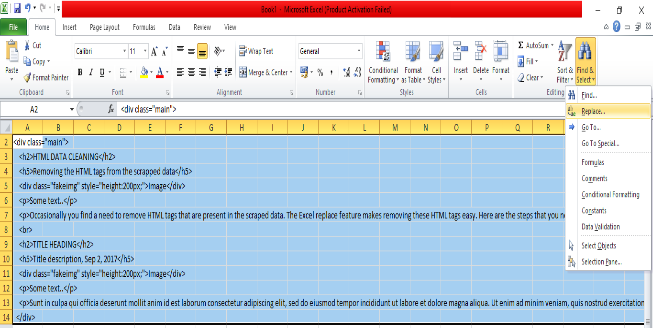
Step 2: In the “Find what” field enter <*>Leave the “Replace with” field blank and then click on the “Replace All” button. All the html tags will be removed.
When you paste data from an external source to an Excel spreadsheet (plain text reports, numbers from web pages, etc.) you are likely to get extra spaces along with important data. There can be leading and trailing spaces, several blanks between words, and thousand separators for numbers.
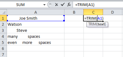
“TRIM” function in Excel is used to remove the white spaces between and at the ends of the words in a cell.
=TRIM(A1)
Step 1: Write the trim function in the new column as shown representing any cell of the column in which the content is to be trimmed and then click on the tick mark as pointed by the arrow


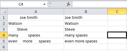
Step 2: The content of the particular cell will be trimmed and written in the cell C1. Now copy that particular cell by clicking CTRL+C and select all the cells below it which are in the same row of the data to be trimmed and press Enter or CTRL+V. Then finally the trimmed data will be displayed in the C column. Finally replace the actual data with the trimmed data.
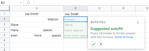
In Google Sheets: Similar steps are used in the Google sheets as well. After entering the formula click on Enter and then a pop up window with suggested autofill will appear then click on tick mark appear in the autofill suggestion window, thus entered column elements will be trimmed.

Converting numbers to number types
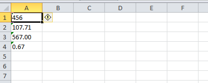
Numbers that are stored as text can cause unexpected results. Select the cells, and then click the Excel Error Alert button to choose a convert option. Or, do the following if that button isn't available.


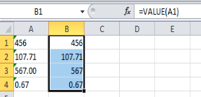
The “VALUE” function does this task of converting numbers in the text format into number types. =VALUE(A1)
STEP 1: Insert a new column next to the cells with text. In this example, column A contains the text stored as numbers. Column B is the new column. In one of the cells of the new column, type =VALUE() and inside the parenthesis, type a cell reference that contains text stored as numbers. In this example it's cell A1.
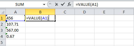


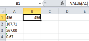
Step 2: Click on the tick mark pointed by an arrow. Then the respective number type will be displayed in the new column. Now copy that particular cell and select the cells below it and press CTRL+V or click “Enter”.
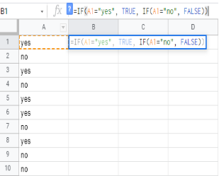
Converting Boolean values Yes->TRUE and No-> False
If you would like to change yes to TRUE and no to FALSE for the data present in the sheet then the “IF” formula is useful. The same is applicable if you want to change Boolean TRUE or FALSE into 1 or 0.
In this example It is shown to convert the yes and no values into TRUE and FALSE respectively.
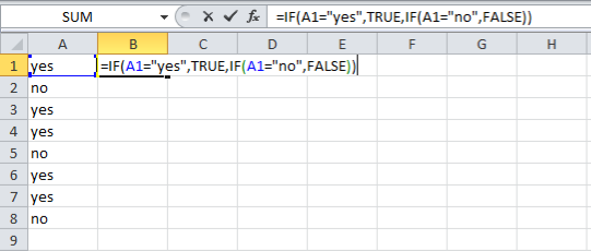
Step 1: Insert a new column next to the cells containing yes or no similar to above operation. In one of the cells of the new column, type
=IF(A1="yes",TRUE,IF(A1="no",FALSE)). 

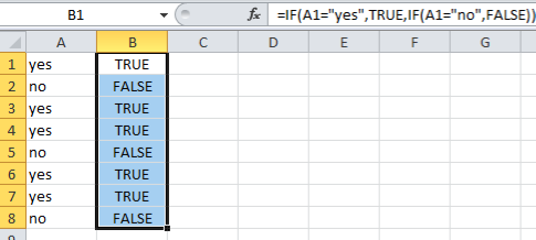
Step 2: : Click on the tick mark pointed by an arrow. Then the respective Boolean type(TRUE / FALSE) will be displayed in the new column. Now copy that particular cell and select the cells below it and press CTRL+V or click “Enter” to convert all the values in the A column into Boolean expressions.
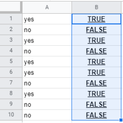
Similar approach is applicable for Google sheets as well.
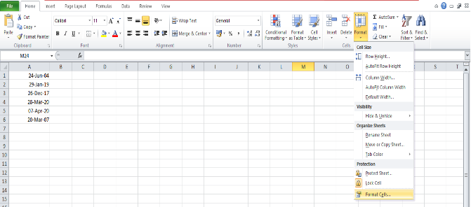
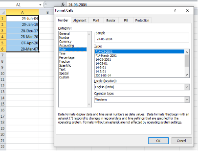
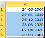
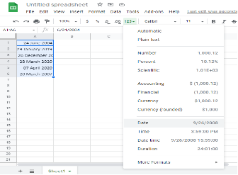
Converting dates to machine-readable formats:
For converting dates into required format an option named “Format Cells” is present which contains a feature to convert the dates into required format.
STEP 1: Select all the data of dates that is to be formatted and click on format scroll button and then select format cells there appears numbers tab.
Step 2 : Select the date and the required date format and then click ok. There it finishes the task and the selected dates will be formatted to selected format.
In the Google sheets to convert the format of date click on the number formats drop down icon and then select the required format based on the choice.


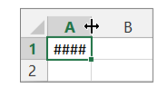
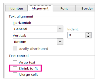
To make the cell content smaller: To make the cell contents smaller, click Home >  next to Alignment, and then check the Shrink to fit box in the Format Cells dialog box.
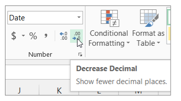
Decrease decimal places: If numbers have too many decimal places, click Home > Decrease Decimal.
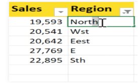
Filtering the data: In the example below, we have a list of salespeople, and each one falls into one of four regions (in column G): North, South, East, or West. If you look closely, you may notice that the regions for Katell Hall and Illana Erickson are misspelled. This could cause problems with certain formulas or PivotTables, so it's important to correct these errors.
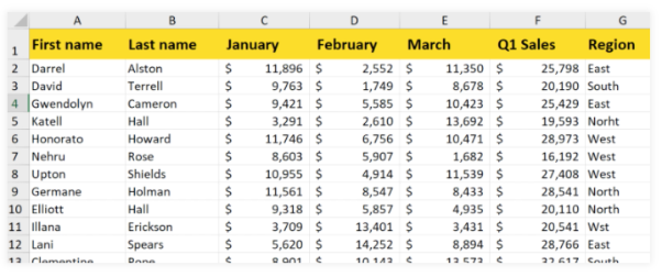
The key to finding the inconsistencies is to create a filter. The filter will allow you to see all of the unique values in the column, making it easier to isolate the incorrect values. In our example, the Region column should only contain the values North, South, East, and West, so any other values will need to be fixed.
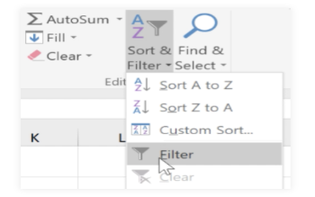
Step1: On the Home tab, go to Sort & Filter > Filter. If your worksheet already has filters, you can skip this step.
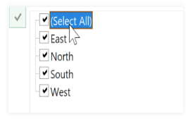
Step 2: Click the filter drop-down arrow in the desired column. A drop-down menu will appear, showing a list of all of the unique values in the column. Deselect all of the correct values, leaving all of the incorrect values selected. In our example, we will deselect North, South, East, and West.
When you're done, click OK.
Step 3: The spread sheet will now be filtered to only show the incorrect values. In our example, there were only a few errors, so we'll fix them manually by typing the correct values for each one. Click the column's filter drop-down arrow again and make sure all of the values listed are correct. When you're done, click Select All, then click OK to show all of the rows.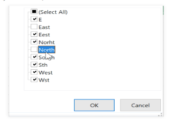
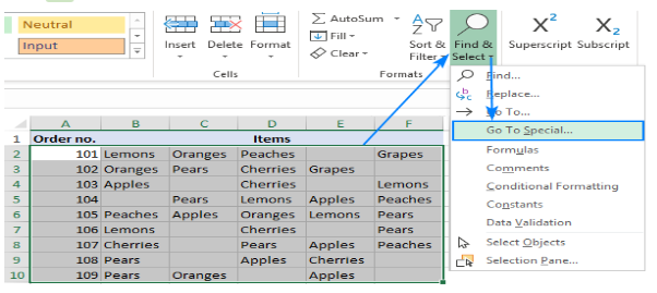
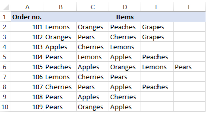
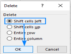
Step 1: Select the range where you want to remove blanks. To quickly select all cells with data, click the upper-left cell and press Ctrl + Shift + End. This will extend the selection to the last used cell. Press F5 and click Special. Or go to the Home tab > Formats group, and click Find & Select > Go to Special.
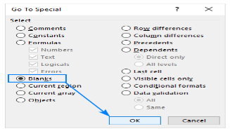
Step 2: In the Go To Special dialog box, select Blanks and click OK. This will select all the blank cells in the range.
Step 3: Right-click any of the selected blanks, and choose Delete… from the context menu.
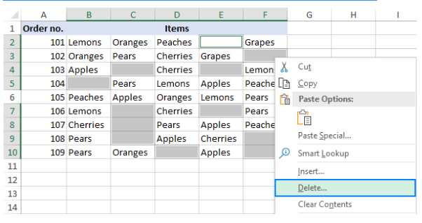
Step 4: Depending on the layout of your data, choose to shift cells left or shift cells up, and click OK. In this example, we go with the first option. That's it. You have successfully removed blank spaces in your table.
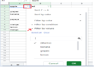
Step 1: Initially select the column that contains data and click on the Data dialog present in the top then select Create a filter from the drop down options. Then a filter icon will appear at the top of the column as shown in the picture.
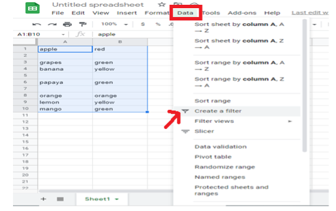
Step 2: Click on the filter icon and then click on filter by values and deselect all the entries except blanks and click OK. All the empty cells will be displayed.
Step 3: Now select all the empty cells and right click on the mouse a pop up will appear. Then click on the Delete Selected rows and all the empty cells will be deleted . Now finally turn off the filter. All the empty cells will be removed. 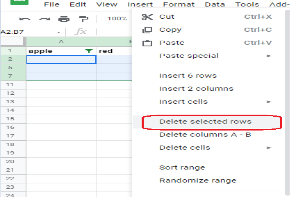
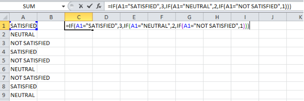
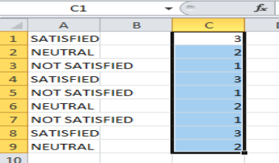
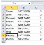
Reviews displayed in the excel sheet can be converted from text to numbers. The IF condition provided in the Excel serves this task.
Take an example of rating on a scale of 3 based on the text mentioned as “Satisfied”, “Neutral”, “Not Satisfied”.
=IF(B1="SATISFIED",3,IF(B1="NEUTRAL",2, IF(B1="NOT SATISFIED",1)))
Step 1: Insert a new column and write the IF() condition as follows and then click on the tick mark pointed by arrow. 

Step 2: Then the numerical rating will be displayed in that particular cell. Copy that and drag down to select all the cells in the column and press CTRL+V or Enter. The numerical rating of the text will be displayed in the C column successfully.
From numbers to text
Similar to above process numerical reviews can be converted to text by using the CHOOSE formula as follows :
=CHOOSE(A1,"NOT SATISFIED","NEUTRAL","SATISFIED")
Before analysing and making decisions based on data in your sheets, it’s important to clean up your data by rectifying errors and improving data consistency. Clean up suggestions will help you do this by surfacing intelligent suggestions in the side panel. These suggestions may include removing extra spaces, removing duplicate rows, adding number formatting, identifying anomalies, fixing inconsistent data, and more. This can help make data clean up faster and more accurate.
To work using Google clean up suggestions. Open the spreadsheet that you want to edit and then click on the Data dialog on the above content bar and then select Cleanup Suggestions in the drop down box. Then there will be certain suggestions given by Google for cleaning the data like identifying duplicate entries, extra white spaces, Empty cells etc.. Based on the requirement of the user one can ignore or implement the cleaning operation based on the suggestions without making any extra efforts to write formulas or check manually.
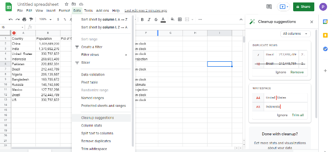

In the above example the cleanup suggestions shown are duplicate entries of Brazil details and extra White Spaces. Based on the requirement you can ignore or implement the suggestion.
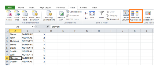
Excel is a package of many advanced features to clean or manipulate the data present in the worksheet. One of those features is removing the duplicate entries.
Step 1: Click any single cell inside the data set. On the Data tab, in the Data Tools group, click Remove Duplicates.
Step 2: A pop up window will be displayed with the columns to be considered while searching for duplicates. If all the columns are to be considered then all the columns should be checked. And then click OK.
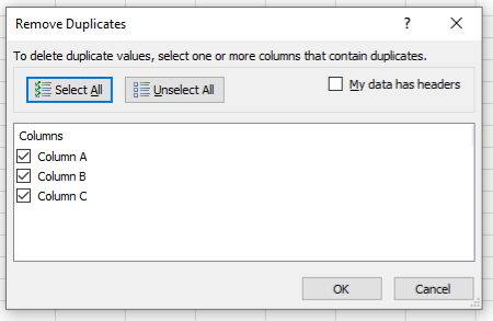
Duplicate entries will be successfully removed.
To change the case of the text present in the sheet the following steps to be done.
Let us consider the sample Worksheet
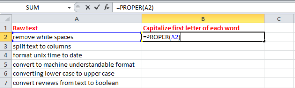
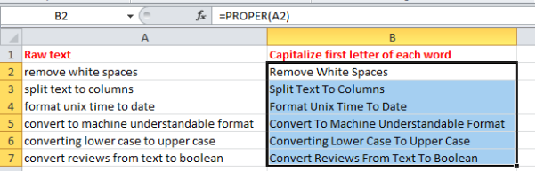
Capitalise first letter of each word
PROPER() function is used for this purpose. Following are the steps to be followed to Capitalize first letter of each word.
Step 1: Insert a new column and write formula =PROPER() and then click on the tick mark indicated by the arrow.

Step 2: The formatted form of text present in the A2 column will be displayed in the B2 column, then copy that(B2) cell and select the cells below it where the formula should be applied and paste by clicking CTRL+V or Enter.
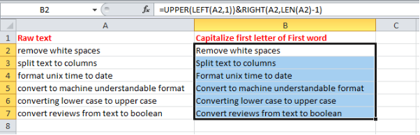
Capitalize only first letter of the first word
There is no inbuilt function for capitalizing only the first word of the first letter. But this can be achieved by the combination of functions.
=UPPER(LEFT(A2,1))&RIGHT(A2,LEN(A2)-1)
The UPPER function is used to capitalise the leftmost letter of the first word and the RIGHT function is used to concatenate the rest of the string to the capitalized first letter.

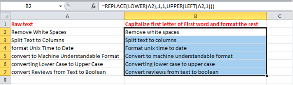
Capitalize the First Letter of the First Word and Change the Rest to Lower Case
Similar to capitalizing the first letter of the first word, this operation also doesn’t contain any inbuilt function. And this also can be achieved using a combination of functions.
=REPLACE(LOWER(A2),1,1,UPPER(LEFT(A2,1)))
Initially the LOWER function converts the entire text into lower case and the UPPER function converts the leftmost letter of the first word into upper case and REPLACE function replaces the lower case first letter lower with upper case one.
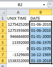
The Unix timestamp tracks time as a running count of seconds. The count begins at the "Unix Epoch" on January 1st, 1970, so a Unix timestamp is simply the total seconds between any given date and the Unix Epoch. Since a day contains 86400 seconds (24 hours x 60 minutes x 60 seconds), conversion to Excel time can be done by dividing days by 86400 and adding the date value for January 1st, 1970.
So, to convert the UNIX timestamp into date a formula is used to convert the seconds into date. The formula is as follows:
=(A2/86400)+DATE(1970,1,1)
In the below example the UNIX time is in column A. The following steps are to be followed to convert UNIX time to date.
Step 1: Insert a new column which consists of a cell with formula to convert the UNIX time to date corresponding to any one of the cells with UNIX time data. Then click on the tick mark pointed by the arrow.

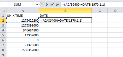

Step 2: The general format value of the date will be displayed. Copy that cell and select all the cells beneath it and press Enter or CTRL+V to change all the UNIX time to general date value.
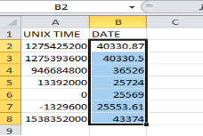
Step 3: Now select the column containing general date values and go to the Number tool bar on the top and change the general to short date or required date format as per the choice from the drop down box.
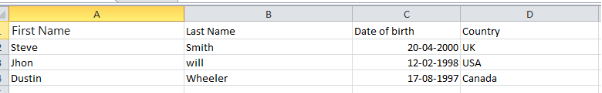
When data is scrapped from a webpage it will be in the form of paragraphs sometimes. Then there will be a need to split the text into different columns based on the requirement.
Let us consider an example with first name, Last name, Date of Birth, Country with all the data in the first column.
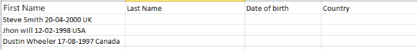
To split this text the steps to be followed are:
Step 1: Initially select the text to be spit and then click on Data on the top dialogue bar and then select Text to columns.
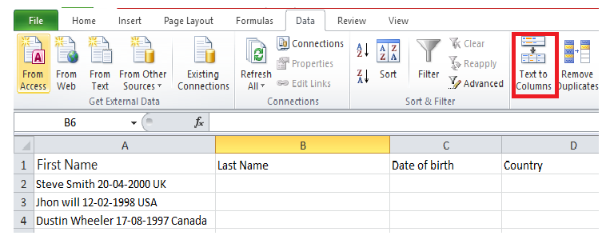
Step 2: Then a pop up window will be displayed. There select the delimited radio button and click Next. In the delimiters checkboxes select the appropriate delimiters. In this case space is selected.
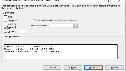
Step 3: Then click next and then click on finish, the text will be spit into four columns as shown.
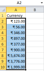
In the Excel sheet there will be a need to change the currency values based on the requirement. To do that there is a feature provided in Excel.
In this section let us initially take a sheet with a column consisting of numbers.
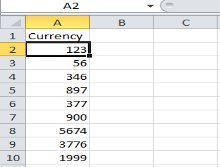
To convert the numbers into currencies the following steps are to be followed
Step 1: Initially go to the home tab and click on the number group.
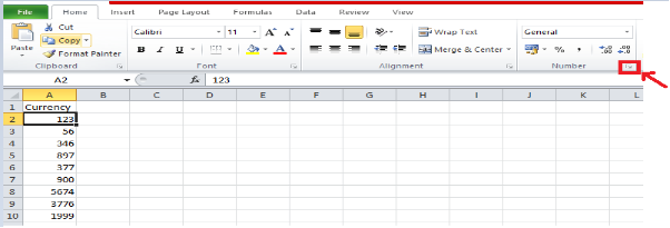
Step 2: A pop up window will be displayed. In the number category select Currency. And then select the appropriate symbol from the drop down list and click OK.
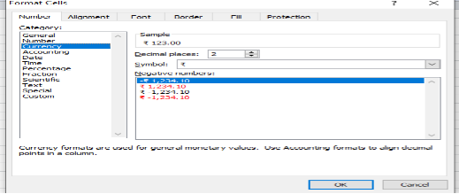
The numbers will be changed into respective currencies. To change the currency, open the above number formatting window and change the symbol of the currency. Then the currency will be changed successfully.

Alot of the times we might need to extract specific text within a block of text as its not always possible to seperate the text using the web scrapiing script
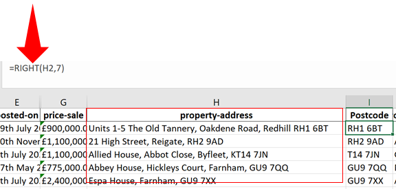
=RIGHT(H2,7)
We aim to make the process of extracting web data quick and efficient so you can focus your resources on what's truly important, using the data to achieve your business goals. In our marketplace, you can choose from hundreds of pre-defined extractors (PDEs) for the world's biggest websites. These pre-built data extractors turn almost any website into a spreadsheet or API with just a few clicks. The best part? We build and maintain them for you so the data is always in a structured form. .
RECENT POSTS
RELATED POSTS
CATEGORIES
follow us on


 Linkedin